

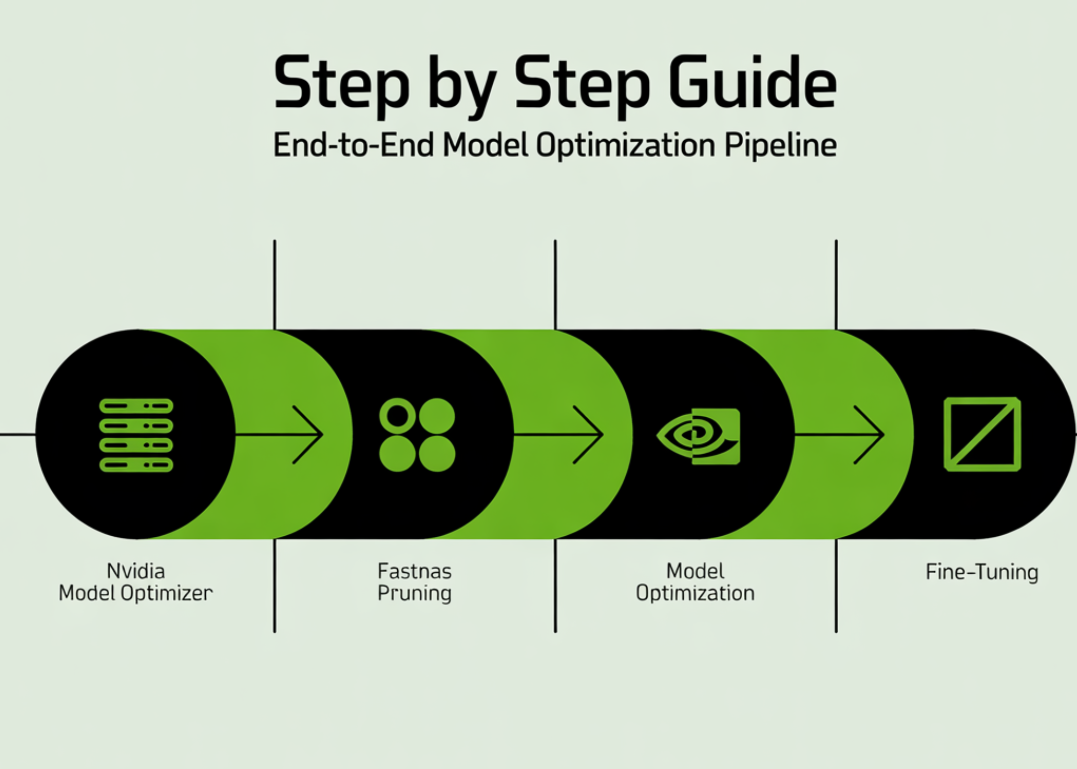

In this tutorial, we build a complete end-to-end pipeline using NVIDIA Model Optimizer to train, prune, and fine-tune a deep learning model directly in Google Colab. We start by setting up the environment and preparing the CIFAR-10 dataset, then define a ResNet architecture and train it to establish a strong baseline. From there, we apply FastNAS pruning to systematically reduce the model’s complexity under FLOPs constraints while preserving performance. We also handle real-world compatibility issues, restore the optimized subnet, and fine-tune it to recover accuracy. By the end, we have a fully working workflow that takes a model from training to deployment-ready optimization, all within a single streamlined setup. Check out the Full Implementation Coding Notebook.
import math
import os
import random
import time
import numpy as np
import torch
import torch.nn as nn
import torch.nn.functional as F
import torchvision
import torchvision.transforms as transforms

from torch.utils.data import DataLoader, Subset
from torchvision.models.resnet import BasicBlock
from tqdm.auto import tqdm
import modelopt.torch.opt as mto
import modelopt.torch.prune as mtp
SEED = 123
random.seed(SEED)
np.random.seed(SEED)
torch.manual_seed(SEED)
if torch.cuda.is_available():
torch.cuda.manual_seed_all(SEED)
FAST_MODE = True
batch_size = 256 if FAST_MODE else 512
baseline_epochs = 20 if FAST_MODE else 120
finetune_epochs = 12 if FAST_MODE else 120
train_subset_size = 12000 if FAST_MODE else None
val_subset_size = 2000 if FAST_MODE else None
test_subset_size = 4000 if FAST_MODE else None
target_flops = 60e6
We begin by installing all required dependencies and importing the necessary libraries to set up our environment. We initialize seeds to ensure reproducibility and configure the device to leverage a GPU if available. We also define key runtime parameters, such as batch size, epochs, dataset subsets, and FLOP constraints, to control the overall experiment.
worker_seed = SEED + worker_id
np.random.seed(worker_seed)
random.seed(worker_seed)
def build_cifar10_loaders(train_batch_size=256,
train_subset_size=None,
val_subset_size=None,
test_subset_size=None):
normalize = transforms.Normalize(
mean=[0.4914, 0.4822, 0.4465],
std=[0.2470, 0.2435, 0.2616],
)
train_transform = transforms.Compose([
transforms.ToTensor(),
transforms.RandomHorizontalFlip(),
transforms.RandomCrop(32, padding=4),
normalize,
])
eval_transform = transforms.Compose([
transforms.ToTensor(),
normalize,
])
train_full = torchvision.datasets.CIFAR10(
root=”./data”, train=True, transform=train_transform, download=True
)
val_full = torchvision.datasets.CIFAR10(
root=”./data”, train=True, transform=eval_transform, download=True
)
test_full = torchvision.datasets.CIFAR10(
root=”./data”, train=False, transform=eval_transform, download=True
)
n_trainval = len(train_full)
ids = np.arange(n_trainval)
np.random.shuffle(ids)
n_train = int(n_trainval * 0.9)
train_ids = ids[:n_train]
val_ids = ids[n_train:]
if train_subset_size is not None:
train_ids = train_ids[:min(train_subset_size, len(train_ids))]
if val_subset_size is not None:
val_ids = val_ids[:min(val_subset_size, len(val_ids))]
test_ids = np.arange(len(test_full))
if test_subset_size is not None:
test_ids = test_ids[:min(test_subset_size, len(test_ids))]
train_ds = Subset(train_full, train_ids.tolist())
val_ds = Subset(val_full, val_ids.tolist())
test_ds = Subset(test_full, test_ids.tolist())
num_workers = min(2, os.cpu_count() or 1)
g = torch.Generator()
g.manual_seed(SEED)
train_loader = DataLoader(
train_ds,
batch_size=train_batch_size,
shuffle=True,
num_workers=num_workers,
pin_memory=torch.cuda.is_available(),
worker_init_fn=seed_worker,
generator=g,
)
val_loader = DataLoader(
val_ds,
batch_size=512,
shuffle=False,
num_workers=num_workers,
pin_memory=torch.cuda.is_available(),
worker_init_fn=seed_worker,
)
test_loader = DataLoader(
test_ds,
batch_size=512,
shuffle=False,
num_workers=num_workers,
pin_memory=torch.cuda.is_available(),
worker_init_fn=seed_worker,
)
print(f”Train: {len(train_ds)} | Val: {len(val_ds)} | Test: {len(test_ds)}”)
return train_loader, val_loader, test_loader
train_loader, val_loader, test_loader = build_cifar10_loaders(
train_batch_size=batch_size,
train_subset_size=train_subset_size,
val_subset_size=val_subset_size,
test_subset_size=test_subset_size,
)
We construct the full data pipeline by preparing CIFAR-10 datasets with appropriate augmentations and normalization. We split the dataset to reduce its size and speed up experimentation. We then create efficient data loaders that ensure proper batching, shuffling, and reproducible data handling.
if isinstance(m, (nn.Linear, nn.Conv2d)):
nn.init.kaiming_normal_(m.weight)
class LambdaLayer(nn.Module):
def __init__(self, lambd):
super().__init__()
self.lambd = lambd
def forward(self, x):
return self.lambd(x)
class ResNet(nn.Module):
def __init__(self, num_blocks, num_classes=10):
super().__init__()
self.in_planes = 16
self.layers = nn.Sequential(
nn.Conv2d(3, 16, kernel_size=3, stride=1, padding=1, bias=False),
nn.BatchNorm2d(16),
nn.ReLU(),
self._make_layer(16, num_blocks, stride=1),
self._make_layer(32, num_blocks, stride=2),
self._make_layer(64, num_blocks, stride=2),
nn.AdaptiveAvgPool2d((1, 1)),
nn.Flatten(),
nn.Linear(64, num_classes),
)
self.apply(_weights_init)
def _make_layer(self, planes, num_blocks, stride):
strides = [stride] + [1] * (num_blocks – 1)
layers = []
for s in strides:
downsample = None
if s != 1 or self.in_planes != planes:
downsample = LambdaLayer(
lambda x: F.pad(
x[:, :, ::2, ::2],
(0, 0, 0, 0, planes // 4, planes // 4),
“constant”,
0,
)
)
layers.append(BasicBlock(self.in_planes, planes, s, downsample))
self.in_planes = planes
return nn.Sequential(*layers)
def forward(self, x):
return self.layers(x)
def resnet20():
return ResNet(num_blocks=3).to(device)
We define the ResNet20 architecture from scratch, including custom initialization and shortcut handling through lambda layers. We structure the network using convolutional blocks and residual connections to capture hierarchical features. We finally encapsulate the model creation into a reusable function that moves it directly to the selected device.
def __init__(self, optimizer, warmup_steps, decay_steps, warmup_lr=0.0, last_epoch=-1):
self.warmup_steps = warmup_steps
self.warmup_lr = warmup_lr
self.decay_steps = max(decay_steps, 1)
super().__init__(optimizer, last_epoch)
def get_lr(self):
if self.last_epoch < self.warmup_steps:
return [
(base_lr – self.warmup_lr) * self.last_epoch / max(self.warmup_steps, 1) + self.warmup_lr
for base_lr in self.base_lrs
]
current_steps = self.last_epoch – self.warmup_steps
return [
0.5 * base_lr * (1 + math.cos(math.pi * current_steps / self.decay_steps))
for base_lr in self.base_lrs
]
def get_optimizer_scheduler(model, lr, weight_decay, warmup_steps, decay_steps):
optimizer = torch.optim.SGD(
filter(lambda p: p.requires_grad, model.parameters()),
lr=lr,
momentum=0.9,
weight_decay=weight_decay,
)
scheduler = CosineLRwithWarmup(optimizer, warmup_steps, decay_steps)
return optimizer, scheduler
def loss_fn_default(model, outputs, labels):
return F.cross_entropy(outputs, labels)
def train_one_epoch(model, loader, optimizer, scheduler, loss_fn=loss_fn_default):
model.train()
running_loss = 0.0
total = 0
for images, labels in loader:
images = images.to(device, non_blocking=True)
labels = labels.to(device, non_blocking=True)
outputs = model(images)
loss = loss_fn(model, outputs, labels)
optimizer.zero_grad(set_to_none=True)
loss.backward()
optimizer.step()
scheduler.step()
running_loss += loss.item() * labels.size(0)
total += labels.size(0)
return running_loss / max(total, 1)
@torch.no_grad()
def evaluate(model, loader):
model.eval()
correct = 0
total = 0
for images, labels in loader:
images = images.to(device, non_blocking=True)
labels = labels.to(device, non_blocking=True)
logits = model(images)
preds = logits.argmax(dim=1)
correct += (preds == labels).sum().item()
total += labels.size(0)
return 100.0 * correct / max(total, 1)
def train_model(model, train_loader, val_loader, epochs, ckpt_path,
lr=None, weight_decay=1e-4, print_every=1):
if lr is None:
lr = 0.1 * batch_size / 128
steps_per_epoch = len(train_loader)
warmup_steps = max(1, 2 * steps_per_epoch if FAST_MODE else 5 * steps_per_epoch)
decay_steps = max(1, epochs * steps_per_epoch)
optimizer, scheduler = get_optimizer_scheduler(
model=model,
lr=lr,
weight_decay=weight_decay,
warmup_steps=warmup_steps,
decay_steps=decay_steps,
)
best_val = -1.0
best_epoch = -1
print(f”Training for {epochs} epochs…”)
for epoch in tqdm(range(1, epochs + 1)):
train_loss = train_one_epoch(model, train_loader, optimizer, scheduler)
val_acc = evaluate(model, val_loader)
if val_acc >= best_val:
best_val = val_acc
best_epoch = epoch
torch.save(model.state_dict(), ckpt_path)
if epoch == 1 or epoch % print_every == 0 or epoch == epochs:
print(f”Epoch {epoch:03d} | train_loss={train_loss:.4f} | val_acc={val_acc:.2f}%”)
model.load_state_dict(torch.load(ckpt_path, map_location=device))
print(f”Restored best checkpoint from epoch {best_epoch} with val_acc={best_val:.2f}%”)
return model, best_val
We implement the training utilities, including a cosine learning rate scheduler with warmup, to enable stable optimization. We define loss computation, a training loop for one epoch, and an evaluation function to measure accuracy. We then build a complete training pipeline that tracks the best model and restores it based on validation performance.
baseline_ckpt = “resnet20_baseline.pth”
start = time.time()
baseline_model, baseline_val = train_model(
baseline_model,
train_loader,
val_loader,
epochs=baseline_epochs,
ckpt_path=baseline_ckpt,
lr=0.1 * batch_size / 128,
weight_decay=1e-4,
print_every=max(1, baseline_epochs // 4),
)
baseline_test = evaluate(baseline_model, test_loader)
baseline_time = time.time() – start
print(f”\nBaseline validation accuracy: {baseline_val:.2f}%”)
print(f”Baseline test accuracy: {baseline_test:.2f}%”)
print(f”Baseline training time: {baseline_time/60:.2f} min”)
fastnas_cfg = mtp.fastnas.FastNASConfig()
fastnas_cfg[“nn.Conv2d”][“*”][“channel_divisor”] = 16
fastnas_cfg[“nn.BatchNorm2d”][“*”][“feature_divisor”] = 16
dummy_input = torch.randn(1, 3, 32, 32, device=device)
def score_func(model):
return evaluate(model, val_loader)
search_ckpt = “modelopt_search_checkpoint_fastnas.pth”
pruned_ckpt = “modelopt_pruned_model_fastnas.pth”
import torchprofile.profile as tp_profile
from torchprofile.handlers import HANDLER_MAP
if not hasattr(tp_profile, “handlers”):
tp_profile.handlers = tuple((tuple([op_name]), handler) for op_name, handler in HANDLER_MAP.items())
print(“\nRunning FastNAS pruning…”)
prune_start = time.time()
model_for_prune = resnet20()
model_for_prune.load_state_dict(torch.load(baseline_ckpt, map_location=device))
pruned_model, pruned_metadata = mtp.prune(
model=model_for_prune,
mode=[(“fastnas”, fastnas_cfg)],
constraints={“flops”: target_flops},
dummy_input=dummy_input,
config={
“data_loader”: train_loader,
“score_func”: score_func,
“checkpoint”: search_ckpt,
},
)
mto.save(pruned_model, pruned_ckpt)
prune_elapsed = time.time() – prune_start
pruned_test_before_ft = evaluate(pruned_model, test_loader)
print(f”Pruned model test accuracy before fine-tune: {pruned_test_before_ft:.2f}%”)
print(f”Pruning/search time: {prune_elapsed/60:.2f} min”)
We train the baseline model and evaluate its performance to establish a reference point for optimization. We then configure FastNAS pruning, define constraints, and apply a compatibility patch to ensure proper FLOPs profiling. We execute the pruning process to generate a compressed model and evaluate its performance before fine-tuning.
restored_pruned_model = mto.restore(restored_pruned_model, pruned_ckpt)
restored_test = evaluate(restored_pruned_model, test_loader)
print(f”Restored pruned model test accuracy: {restored_test:.2f}%”)
print(“\nFine-tuning pruned model…”)
finetune_ckpt = “resnet20_pruned_finetuned.pth”
start_ft = time.time()
restored_pruned_model, pruned_val_after_ft = train_model(
restored_pruned_model,
train_loader,
val_loader,
epochs=finetune_epochs,
ckpt_path=finetune_ckpt,
lr=0.05 * batch_size / 128,
weight_decay=1e-4,
print_every=max(1, finetune_epochs // 4),
)
pruned_test_after_ft = evaluate(restored_pruned_model, test_loader)
ft_time = time.time() – start_ft
print(f”\nFine-tuned pruned validation accuracy: {pruned_val_after_ft:.2f}%”)
print(f”Fine-tuned pruned test accuracy: {pruned_test_after_ft:.2f}%”)
print(f”Fine-tuning time: {ft_time/60:.2f} min”)
def count_params(model):
return sum(p.numel() for p in model.parameters())
def count_nonzero_params(model):
total = 0
for p in model.parameters():
total += (p.detach() != 0).sum().item()
return total
baseline_params = count_params(baseline_model)
pruned_params = count_params(restored_pruned_model)
baseline_nonzero = count_nonzero_params(baseline_model)
pruned_nonzero = count_nonzero_params(restored_pruned_model)
print(“\n” + “=” * 60)
print(“FINAL SUMMARY”)
print(“=” * 60)
print(f”Baseline test accuracy: {baseline_test:.2f}%”)
print(f”Pruned test accuracy before finetune: {pruned_test_before_ft:.2f}%”)
print(f”Pruned test accuracy after finetune: {pruned_test_after_ft:.2f}%”)
print(“-” * 60)
print(f”Baseline total params: {baseline_params:,}”)
print(f”Pruned total params: {pruned_params:,}”)
print(f”Baseline nonzero params: {baseline_nonzero:,}”)
print(f”Pruned nonzero params: {pruned_nonzero:,}”)
print(“-” * 60)
print(f”Baseline train time: {baseline_time/60:.2f} min”)
print(f”Pruning/search time: {prune_elapsed/60:.2f} min”)
print(f”Pruned finetune time: {ft_time/60:.2f} min”)
print(“=” * 60)
torch.save(baseline_model.state_dict(), “baseline_resnet20_final_state_dict.pth”)
mto.save(restored_pruned_model, “pruned_resnet20_final_modelopt.pth”)
print(“\nSaved files:”)
print(” – baseline_resnet20_final_state_dict.pth”)
print(” – modelopt_pruned_model_fastnas.pth”)
print(” – pruned_resnet20_final_modelopt.pth”)
print(” – modelopt_search_checkpoint_fastnas.pth”)
@torch.no_grad()
def show_sample_predictions(model, loader, n=8):
model.eval()
class_names = [
“airplane”, “automobile”, “bird”, “cat”, “deer”,
“dog”, “frog”, “horse”, “ship”, “truck”
]
images, labels = next(iter(loader))
images = images[:n].to(device)
labels = labels[:n]
logits = model(images)
preds = logits.argmax(dim=1).cpu()
print(“\nSample predictions:”)
for i in range(len(preds)):
print(f”{i:02d} | pred={class_names[preds[i]]:<10} | true={class_names[labels[i]]}”)
show_sample_predictions(restored_pruned_model, test_loader, n=8)
We restore the pruned model and verify its performance to ensure the pruning process succeeded. We fine-tune the model to recover accuracy lost during pruning and evaluate the final performance. We conclude by comparing metrics, saving artifacts, and running sample predictions to validate the optimized model end-to-end.
In conclusion, we moved beyond theory and built a complete, production-grade model-optimization pipeline from scratch. We saw how a dense model is transformed into an efficient, compute-aware network through structured pruning, and how fine-tuning restores performance while retaining efficiency gains. We developed a strong intuition for FLOP constraints, automated architecture search, and how FastNAS intelligently navigates the trade-off between accuracy and efficiency. Most importantly, we walked away with a powerful, reusable workflow that we can apply to any model or dataset, enabling us to systematically design high-performance models that are not only accurate but also truly optimized for real-world deployment.
Check out the Full Implementation Coding Notebook. Also, feel free to follow us on Twitter and don’t forget to join our 120k+ ML SubReddit and Subscribe to our Newsletter. Wait! are you on telegram? now you can join us on telegram as well.