

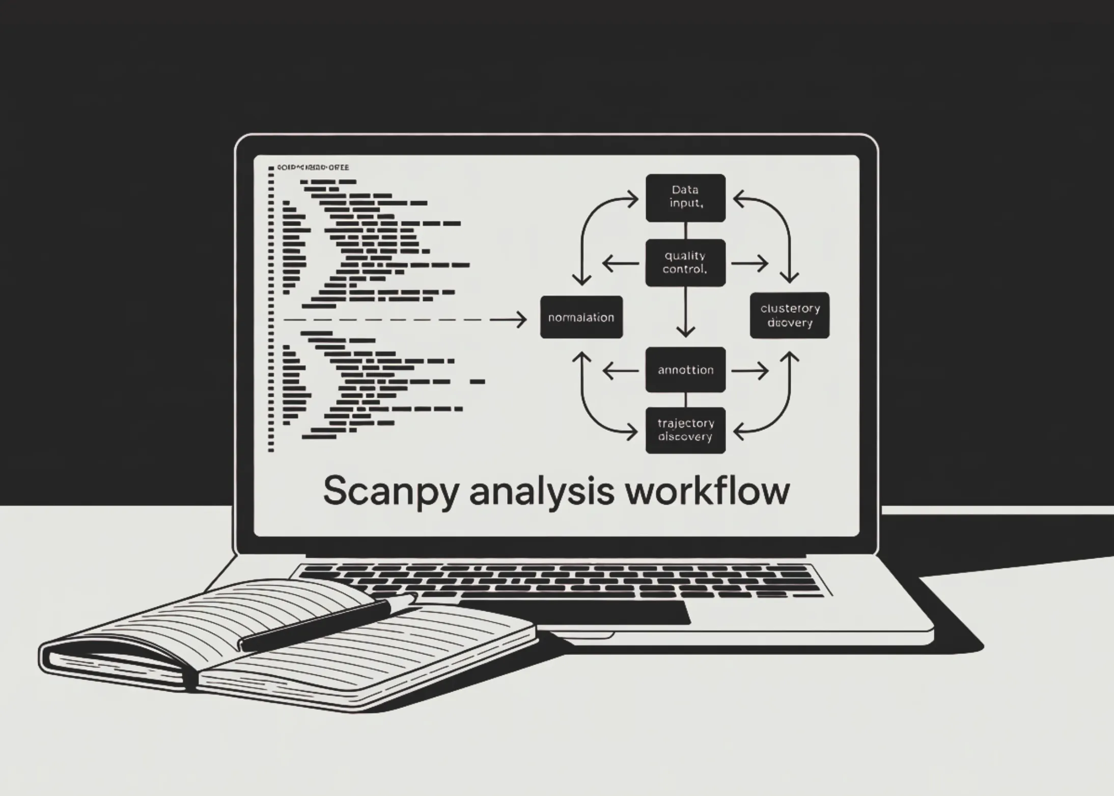

In this tutorial, we perform an advanced single-cell RNA-seq analysis workflow using Scanpy on the PBMC-3k benchmark dataset. We start by loading the dataset, inspecting its structure, and applying quality control checks to evaluate gene counts, total counts, mitochondrial content, and ribosomal gene signals. We then filter low-quality cells and genes, detect potential doublets with Scrublet, normalize the data, apply log transformation, and identify highly variable genes for downstream analysis. Also, we score cell-cycle phases, regress out unwanted technical variation, scale the data, and reduce dimensionality using PCA, UMAP, and t-SNE. We also cluster cells with the Leiden algorithm, identify marker genes, annotate cell populations using canonical PBMC markers, explore trajectory structure with PAGA and diffusion pseudotime, calculate a custom interferon-response score, and finally save the fully analyzed AnnData object for future use.
!pip install -q scanpy leidenalg python-igraph scrublet
import scanpy as sc
import numpy as np
import pandas as pd
import matplotlib.pyplot as plt
import warnings
warnings.filterwarnings(“ignore”)
sc.settings.verbosity = 3
sc.settings.set_figure_params(dpi=80, facecolor=”white”, figsize=(5, 5))
sc.logging.print_header()

adata = sc.datasets.pbmc3k()
adata.var_names_make_unique()
print(adata)
adata.var[“mt”] = adata.var_names.str.startswith(“MT-“)
adata.var[“ribo”] = adata.var_names.str.startswith((“RPS”, “RPL”))
sc.pp.calculate_qc_metrics(
adata, qc_vars=[“mt”, “ribo”], percent_top=None, log1p=False, inplace=True
)
sc.pl.violin(
adata,
[“n_genes_by_counts”, “total_counts”, “pct_counts_mt”],
jitter=0.4, multi_panel=True,
)
sc.pl.scatter(adata, x=”total_counts”, y=”pct_counts_mt”)
sc.pl.scatter(adata, x=”total_counts”, y=”n_genes_by_counts”)
We install the required single-cell analysis libraries and import Scanpy, NumPy, Pandas, Matplotlib, and warning controls. We load the PBMC-3k benchmark dataset, make gene names unique, and inspect the AnnData object structure. We then calculate quality control metrics for mitochondrial and ribosomal genes and visualize count-level quality patterns using violin and scatter plots.
sc.pp.filter_cells(adata, min_genes=200)
sc.pp.filter_genes(adata, min_cells=3)
adata = adata[adata.obs.n_genes_by_counts < 2500, :].copy()
adata = adata[adata.obs.pct_counts_mt < 5, :].copy()
sc.pp.scrublet(adata)
print(“Predicted doublets:”, int(adata.obs[“predicted_doublet”].sum()))
adata = adata[~adata.obs[“predicted_doublet”], :].copy()
adata.layers[“counts”] = adata.X.copy()
sc.pp.normalize_total(adata, target_sum=1e4)
sc.pp.log1p(adata)
sc.pp.highly_variable_genes(adata, min_mean=0.0125, max_mean=3, min_disp=0.5)
sc.pl.highly_variable_genes(adata)
adata.raw = adata
adata = adata[:, adata.var.highly_variable].copy()
We filter out low-quality cells and rarely detected genes to improve the reliability of the dataset. We use Scrublet through Scanpy to identify predicted doublets and remove them before deeper analysis. We then preserve raw counts, normalize expression values, apply log transformation, select highly variable genes, and keep only the most informative features.
s_genes = [“MCM5″,”PCNA”,”TYMS”,”FEN1″,”MCM2″,”MCM4″,”RRM1″,”UNG”,”GINS2″,
“MCM6″,”CDCA7″,”DTL”,”PRIM1″,”UHRF1″,”HELLS”,”RFC2″,”NASP”,
“RAD51AP1″,”GMNN”,”WDR76″,”SLBP”,”CCNE2″,”UBR7″,”POLD3″,”MSH2″,
“ATAD2″,”RAD51″,”RRM2″,”CDC45″,”CDC6″,”EXO1″,”TIPIN”,”DSCC1″,
“BLM”,”CASP8AP2″,”USP1″,”CLSPN”,”POLA1″,”CHAF1B”,”E2F8″]
g2m_genes = [“HMGB2″,”CDK1″,”NUSAP1″,”UBE2C”,”BIRC5″,”TPX2″,”TOP2A”,”NDC80″,
“CKS2″,”NUF2″,”CKS1B”,”MKI67″,”TMPO”,”CENPF”,”TACC3″,”SMC4″,
“CCNB2″,”CKAP2L”,”CKAP2″,”AURKB”,”BUB1″,”KIF11″,”ANP32E”,
“TUBB4B”,”GTSE1″,”KIF20B”,”HJURP”,”CDCA3″,”CDC20″,”TTK”,
“CDC25C”,”KIF2C”,”RANGAP1″,”NCAPD2″,”DLGAP5″,”CDCA2″,”CDCA8″,
“ECT2″,”KIF23″,”HMMR”,”AURKA”,”PSRC1″,”ANLN”,”LBR”,”CKAP5″,
“CENPE”,”NEK2″,”G2E3″,”CBX5″,”CENPA”]
s_genes = [g for g in s_genes if g in adata.var_names]
g2m_genes = [g for g in g2m_genes if g in adata.var_names]
sc.tl.score_genes_cell_cycle(adata, s_genes=s_genes, g2m_genes=g2m_genes)
sc.pp.regress_out(adata, [“total_counts”, “pct_counts_mt”])
sc.pp.scale(adata, max_value=10)
sc.tl.pca(adata, svd_solver=”arpack”)
sc.pl.pca_variance_ratio(adata, log=True, n_pcs=50)
sc.pp.neighbors(adata, n_neighbors=10, n_pcs=40)
sc.tl.umap(adata)
sc.tl.tsne(adata, n_pcs=40)
We define S-phase and G2/M-phase marker genes and retain only those present in the dataset. We score each cell for cell-cycle phase, regress out unwanted variation from total counts and mitochondrial percentage, and scale the data for downstream modeling. We then run PCA, inspect explained variance, construct the neighborhood graph, and generate UMAP and t-SNE embeddings.
sc.tl.leiden(adata, resolution=0.5, flavor=”igraph”, n_iterations=2, directed=False)
sc.pl.umap(adata, color=”leiden”, legend_loc=”on data”, title=”Leiden clusters”)
sc.pl.tsne(adata, color=”leiden”, legend_loc=”on data”, title=”t-SNE clusters”)
sc.tl.rank_genes_groups(adata, “leiden”, method=”wilcoxon”)
sc.pl.rank_genes_groups(adata, n_genes=20, sharey=False)
result = adata.uns[“rank_genes_groups”]
groups = result[“names”].dtype.names
top_df = pd.DataFrame({g: result[“names”][g][:10] for g in groups})
print(“\nTop 10 markers per cluster:\n”, top_df)
marker_genes = {
“B-cell”: [“CD79A”, “MS4A1”],
“CD8 T-cell”: [“CD8A”, “CD8B”],
“CD4 T-cell”: [“IL7R”, “CD4”],
“NK”: [“GNLY”, “NKG7”],
“CD14 Monocyte”: [“CD14”, “LYZ”],
“FCGR3A Monocyte”: [“FCGR3A”, “MS4A7”],
“Dendritic”: [“FCER1A”, “CST3”],
“Megakaryocyte”: [“PPBP”],
}
sc.pl.dotplot(adata, marker_genes, groupby=”leiden”, standard_scale=”var”)
sc.pl.stacked_violin(adata, marker_genes, groupby=”leiden”, swap_axes=True)
We apply Leiden clustering to group cells based on the neighborhood graph and visualize the clusters on UMAP and t-SNE plots. We perform differential expression analysis using the Wilcoxon test to identify the top marker genes for each cluster. We then use canonical PBMC marker genes to support cell-type annotation through dot plots and stacked violin plots.
sc.tl.paga(adata, groups=”leiden”)
sc.pl.paga(adata, color=”leiden”, threshold=0.1)
sc.tl.umap(adata, init_pos=”paga”)
sc.pl.umap(adata, color=”leiden”, legend_loc=”on data”)
sc.tl.diffmap(adata)
sc.pp.neighbors(adata, n_neighbors=10, use_rep=”X_diffmap”)
adata.uns[“iroot”] = np.flatnonzero(adata.obs[“leiden”] == adata.obs[“leiden”].cat.categories[0])[0]
sc.tl.dpt(adata)
sc.pl.umap(adata, color=[“leiden”, “dpt_pseudotime”], legend_loc=”on data”)
ifn_genes = [“ISG15”, “IFI6”, “IFIT1”, “IFIT3”, “MX1”, “OAS1”, “STAT1”, “IRF7″]
ifn_genes = [g for g in ifn_genes if g in adata.raw.var_names]
sc.tl.score_genes(adata, gene_list=ifn_genes, score_name=”IFN_score”)
sc.pl.umap(adata, color=”IFN_score”, cmap=”viridis”)
adata.write(“pbmc3k_analyzed.h5ad”)
print(“\n Analysis complete — saved to pbmc3k_analyzed.h5ad”)
print(adata)
We run PAGA to model connectivity between Leiden clusters and reinitialize UMAP using the PAGA graph to obtain a clearer trajectory structure. We compute diffusion maps and diffusion pseudotime to explore possible progression patterns across cell states. We also calculate an interferon-response gene-set score, visualize it on UMAP, and save the final analyzed object as an .h5ad file.
In conclusion, we built an end-to-end Scanpy pipeline for single-cell RNA-seq analysis, transforming raw PBMC data into interpretable biological insights. We cleaned and preprocessed the dataset, removed noisy cells and doublets, selected informative genes, and generated meaningful embeddings to visualize cellular structure. We then used Leiden clustering and differential expression analysis to discover marker genes and connect clusters to known immune cell types. By adding PAGA, diffusion pseudotime, and custom gene-set scoring, we extended the workflow beyond basic clustering and showed how Scanpy supports deeper biological interpretation. At last, we had a saved .h5ad object that contains the processed data, annotations, scores, clusters, and visual analysis results, ready for downstream exploration or reporting.
Check out the Full Codes with Notebook here. Also, feel free to follow us on Twitter and don’t forget to join our 150k+ ML SubReddit and Subscribe to our Newsletter. Wait! are you on telegram? now you can join us on telegram as well.
Need to partner with us for promoting your GitHub Repo OR Hugging Face Page OR Product Release OR Webinar etc.? Connect with us
The post How to Build a Single-Cell RNA-seq Analysis Pipeline with Scanpy for PBMC Clustering, Annotation, and Trajectory Discovery appeared first on MarkTechPost.